Accelerating structures for efficient intersection computation

summary

This section discusses the different accelerating structures used to efficiently compute the intersections of the rays with the scene.

The intersection computation problem

The ray tracing simulation needs to find the obstacle encountered by every ray. The naive approach consists in performing intersection tests between every ray and all the primitives of the scene. For a single ray, the complexity of this algorithm is O(N) where N is the number of primitives. Though this is acceptable for small scenes, this is too costly in realistic scenarios where scenes are composed of tens of thousands of triangles.

For this reason, a lot of efforts have been put into designing structures that can reduce the complexity of computing intersections of a ray with the primitives of a scene. The idea is to organize the primitives in such a way that it is not necessary to perform intersection tests for all of them.

The overhead of building these accelerating structures can be done with O(N x log(N)) complexity. Then, they can be used for each ray to compute intersections in O(log(N)).

Most of the information on this page comes from Mathieau Dreher’s Master thesis (ref: Développement d’un lancer de rayons 3D générique pour l’acoustique et intégration dans Tympan. Mathieu Dreher 2011)

The different kinds of accelerating structures implemented in code Tympan

Brute force

The brute force accelerator corresponds to the naive approach of testing each primitives of the scene for intersection. It is used to find intersections with receptors wich are placed in a seperate scene.

Uniform grid

This approach consists in dividing the scene in a uniform grid of cells also called voxels. Each time the ray enters a new voxel an intersection test is performed on each primitive in the cell. Once all the primitives in a cell have been tested, the algorithm moves on to the neighboring which is determined by the side from which the ray exited the current cell.

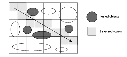
Uniform grid traversed by a ray

The main advantages of this approach is that it is conceptually easy to understand and given any primitive we can quickly find which cell(s) it belongs to when building the grid.

The drawback of this method is that the different cells can contain a very different amount of primitives. In the most extreme case, all cells are empty except one that contains all the primitives. Another problem is that primitives can belong to several cells. This can result in the same primitive being tested multiple time for intersection.

Although the worst case scenario is unlikely, the triangulation algorithm used to build the scene tends to produce triangles of very different sizes. Indeed, flat regions will be composed of big triangles whereas the surroundings of buildings will be made of many small ones.

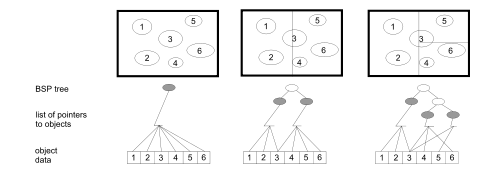
Bounding Volume Hierarchy

The Bounding Volume Hierarchy (BVH) is an adaptive structure that uses a tree to build a hierarchy of bounding boxes. Instead of dividing the space of the scene like the Uniform Grid approach, this strategy divides the set of primitives.

This structure is built as follows:

• We first create the root of the tree which contains all primitives

• Then, we create two children by splitting the list of primitives of the current node in two sublists

• The process is applied recursively until some stoping criterion is met (number of primitives per leaves or maximum tree depth)

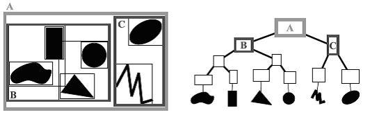
Representation of primitives in a hierachy of bounding volumes

Finding the primitives intersected by the ray is done by, starting at the root node, following the branches of the tree as long as the ray intersects the corresponding bounding boxes. When a leaf is reached, intersection tests are performed between the ray and the primitives contained in the sublist.

The list of primitives of each node can be split according to different strategies:

• Split the volume in the middle of one of its axes (usually we pick the biggest axis)

• Split the list of primitives around its median

• Split the list of primitives according to some cost function (e.g Surface Area Heuristic)

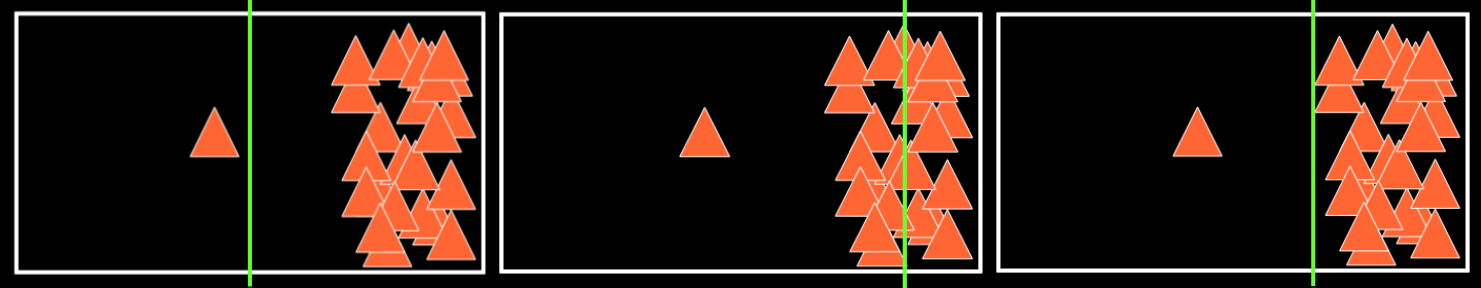
Split strategies - Left: Middle split, Center: Median split, Right: SAH split

The BVH accelerating structure as the advantage of being adaptive, not creating any empty node and only containing one instance of each primitive.

Its drawbacks are that the bounding boxes of different nodes can overlap. This means that the traversal cannot be stopped at the first intersection encountered because a closer one might be discovered when exploring the rest of the tree. Also, the size of the bounding boxes depends on the size of the primitives, which means that big triangles will have big bounding boxes. This creates big leaves and big internal nodes increasing the likelihood of the traversal engaging in parts of the tree for which there are no real intersections to be found.

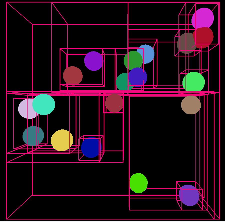
Example of subdivision of the volume with 10 spheres using the median

Kd-tree

The Kd-tree accelerating structure is very similar to the BVH, but instead of dividing the set of primitives id divides the space. Indeed, each node of the tree is split into two smaller ones by dividing the volume of the current one in two parts according to some plan carried by one of the canonical axes.

As for the BVH approach, the position of the dividing plan can be determined through 3 different strategies:

• Sort the primitives of a node along one of the axes and use the position of the median primitive

• Take the middle of the biggest axis

• Use a cost function such as the Surface Area Heuristic (SAH)

Example of a kd-tree using with the middle split strategy

Unlike the BVH approach, a Kd-tree can contain multiple references to the same primitive (if it crosses one of the dividing plans). The main advantage of this approach is to be adaptive while still allowing a front-to-back traversal (i.e, the traversal can be stopped at the first intersection encountered).

The kd-tree is built recursively. This implies that every sub-tree must be constructed before picking the most efficient structure. In practice, a lot of approximations chose to consider that only a simple leaf is added instead of a sub-tree, hence avoiding to deal with the recursion.

Though is construction time is considered by some to be to heavy, the kd-tree is regarded as the optimal accelerating structure for offline rendering (ref: Vlastimil Havran. Heuristic Ray Shooting Algorithms. Ph.d. thesis, Department of Computer Science and Engineering, Faculty of Electrical Engineering, Czech Technical University in Prague, November 2000).

Surface Area Heuristic

The Surface Area Heuristic is based on the idea that, for an infinite amount of rays, the probability of hitting a particular volume is proportional to its area. It uses the area of the primitives contained in a node to estimate where the dividing plan should be put in order to minimise the cost of traversal.

The cost of a particular sub-tree corresponds to the cost of traversing the node (e.g bounding box intersection) plus the cost of intersecting its two children weighted by their probability of being hit by a ray. It is computed with the following formula:

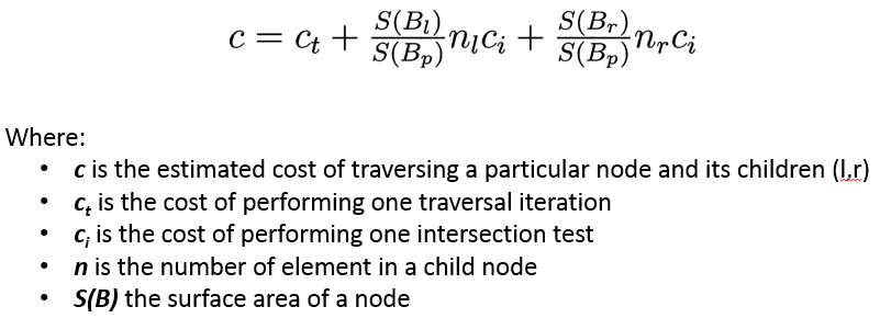
This cost function gives us a criterion to stop building the tree: a node is split in two if the cost of adding two sub-trees is higher than the cost of adding a leaf.

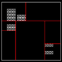
Example of a subdivision of the space with a kd-tree using the SAH cost function